Expert parallelism at hero scale

Summary

• Expert Parallelism (EP) unlocked a ~50% larger model at the same ~23B active size (535B vs 360B total).

• The hero run used our fixed-capacity EP kernel on an NVL72 cluster, reaching 21.5% model FLOPs utilization (MFU) with a 3.4% token-expert assignment drop rate.

The path to our EP configuration led through Fully Sharded Data Parallel (FSDP), off-the-shelf and custom kernels. Each option trades off token drop rate, throughput, and model capacity. Below is an account of our journey.

Why MoE?

We use MoE because it provides greater model capacity for a given compute budget.

In our Delphi work, we established a method for dense model selection through small-scale experiments and scaling recipes. The Quantile Balancing experiment validated a Mixture of Experts (MoE) with 32B total and 5B active parameters through 326B tokens.

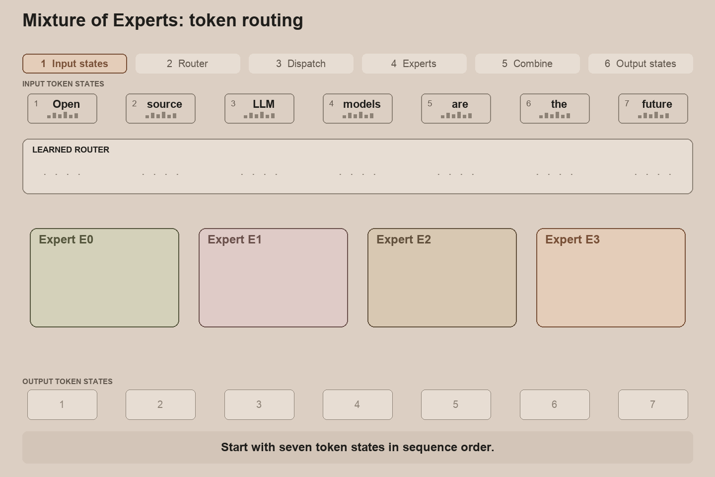
MoE activates only a subset of its experts’ weights for each token. This allows total parameter count to increase without a proportional increase in computation per token. Compared with a dense model of similar total parameter count, an MoE generally requires fewer floating-point operations (FLOPs) per token. That reduction allows more training tokens within a fixed FLOP budget. In practice, the benefit also depends on communication costs, padding, and kernel efficiency.

Why shard?

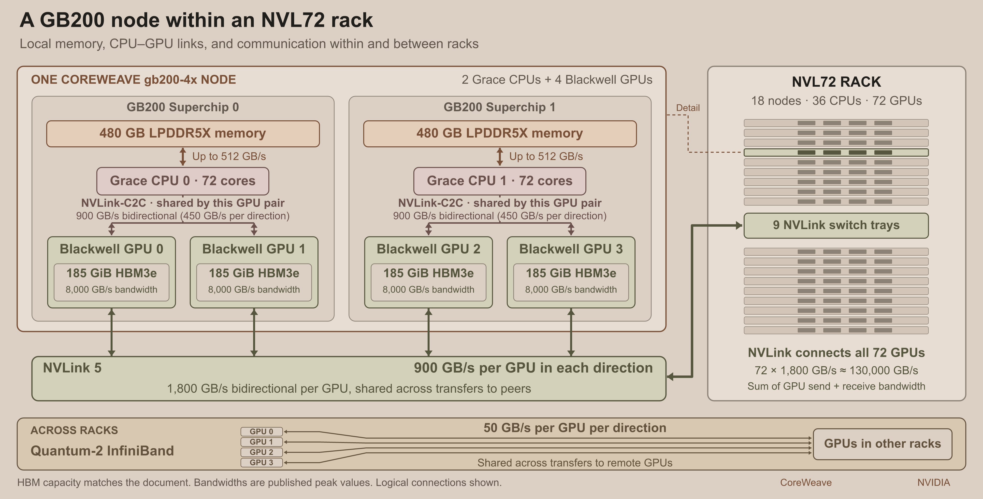
Transformer training relies on efficient matrix multiplications, which require the operands and outputs to fit in the accelerator’s HBM. For example, with BF16 and FP32 mixed precision and an Adam optimizer, model state uses 16 bytes per parameter. A 535B model therefore requires almost 8 TiB for BF16 weights, BF16 gradients, FP32 master weights, and FP32 optimizer states. This excludes activations, communication buffers, and other overhead. That exceeds the 185 GiB available on a single B200. We must use multiple accelerators and distribute the model across them.

Sharding means splitting weights or activations across multiple accelerators. Data Parallelism (DP), Fully Sharded Data Parallel (FSDP), and Expert Parallelism (EP) are three of many possible parallelism methods. See How To Scale Your Model: Sharding for more details. In practice, these methods are often combined to meet hardware and model constraints.

View the full hardware diagram.

Sharding across nodes or racks introduces communication, and its cost depends on the interconnect. Communication within a device, node, or NVLink domain is faster than communication across racks through InfiniBand. Our training setup uses NVL72 racks, with a guaranteed allocation of 16 nodes per rack and four B200s per node. Within a rack, each GPU has up to 900 GB/s of NVLink bandwidth in each direction, shared across transfers to other GPUs. InfiniBand connects the racks at 50 GB/s per GPU in each direction, one eighteenth of the NVLink bandwidth. An NVL72 rack with 72 GPUs is considered healthy when 64 GPUs are online¹, and thus we can assume a single rack has 11.6 TiB of HBM.

FSDP and its limits

The next question is how to shard the model. Data Parallelism (DP) splits the training batch across GPUs. For a fixed global batch, each GPU processes fewer tokens, which reduces activation memory per GPU. However, ordinary DP keeps a complete copy of the parameters, gradients, and optimizer state on each GPU. If that model state exceeds one GPU’s memory, DP alone cannot solve the problem.

FSDP supports larger models by splitting weights, gradients, and optimizer state across GPUs. Each GPU processes a different shard of the batch. Before computing a layer, the GPUs gather the weights so each GPU can process its own tokens. During backward computation, each GPU calculates gradients from those tokens. The GPUs then combine these gradients and distribute the resulting shards to the GPUs that update the corresponding weights. FSDP scales to larger models at the cost of network communication.

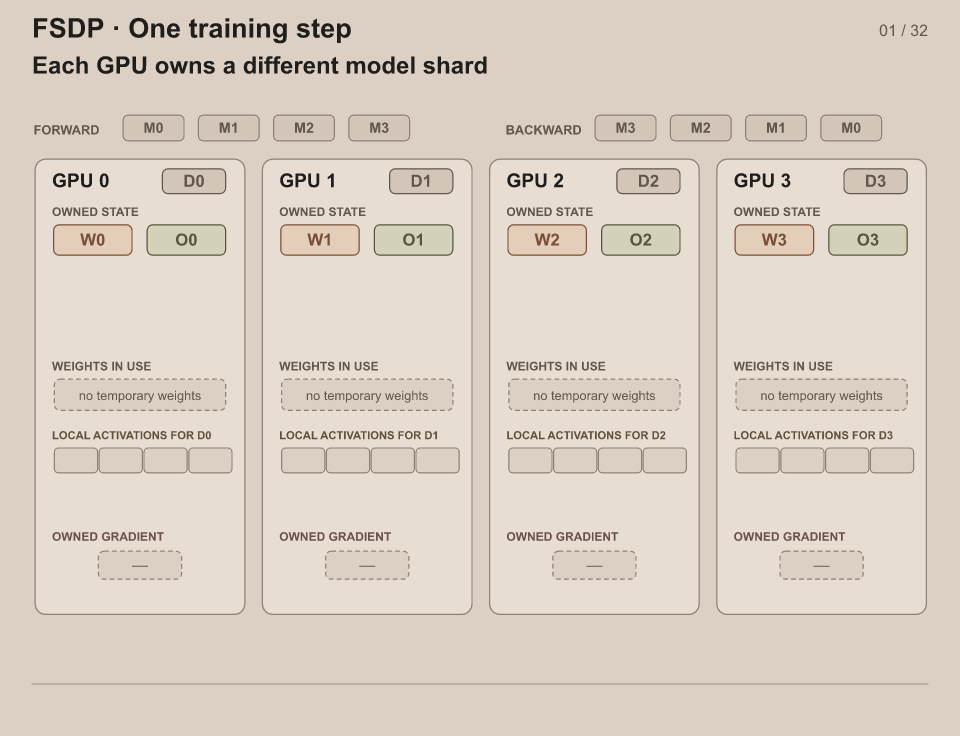
The memory capacity and interconnect bandwidth of an NVL72 rack allow efficient FSDP-only training of large models. Our initial plan was to train a 360B-A23B model with FSDP alone, the largest model we could fit on a single rack in our setup. We then considered whether we could increase model capacity further.

As total model size increases, FSDP encounters several constraints:

• The model can exceed the memory capacity of one NVLink domain. With the same batch size and memory strategy, this requires communication across racks, which increases communication costs.

• A single layer’s weights and activations can exceed the memory available on an accelerator, leading to Out Of Memory (OOM) errors.

• Transferring activations can become more efficient than transferring weights. At that point, EP can be more efficient than FSDP for expert MLP weights. See How To Scale Your Model: Transformer Accounting for more details.

Interconnect bandwidth has a substantial effect on FSDP efficiency. Sharding across racks increases communication costs because InfiniBand bandwidth is approximately an order of magnitude lower than NVLink bandwidth within a rack. Where possible, GPUs can perform other computations during these transfers. This is called communication/computation overlap.

Why EP?

As we scale up the MoE model capacity from small experiments to the hero shape, fairly quickly routed expert MLP weights account for most of the weights. In the 360B total parameter model, roughly 97% of the weights are the expert MLP weights. In vanilla FSDP, each GPU gathers the expert weights before computation. These temporary weights add to the memory required for optimizer state, gradients, and activations.

EP keeps expert weights partitioned across GPUs. It transfers token representations to the GPUs that own the selected experts, then returns their outputs. Since EP does not require gathering all expert weights, it also unlocks larger total capacity model shapes. EP unlocked the 535B-A23B shape, a roughly 50% larger model at the same ~23B active size.

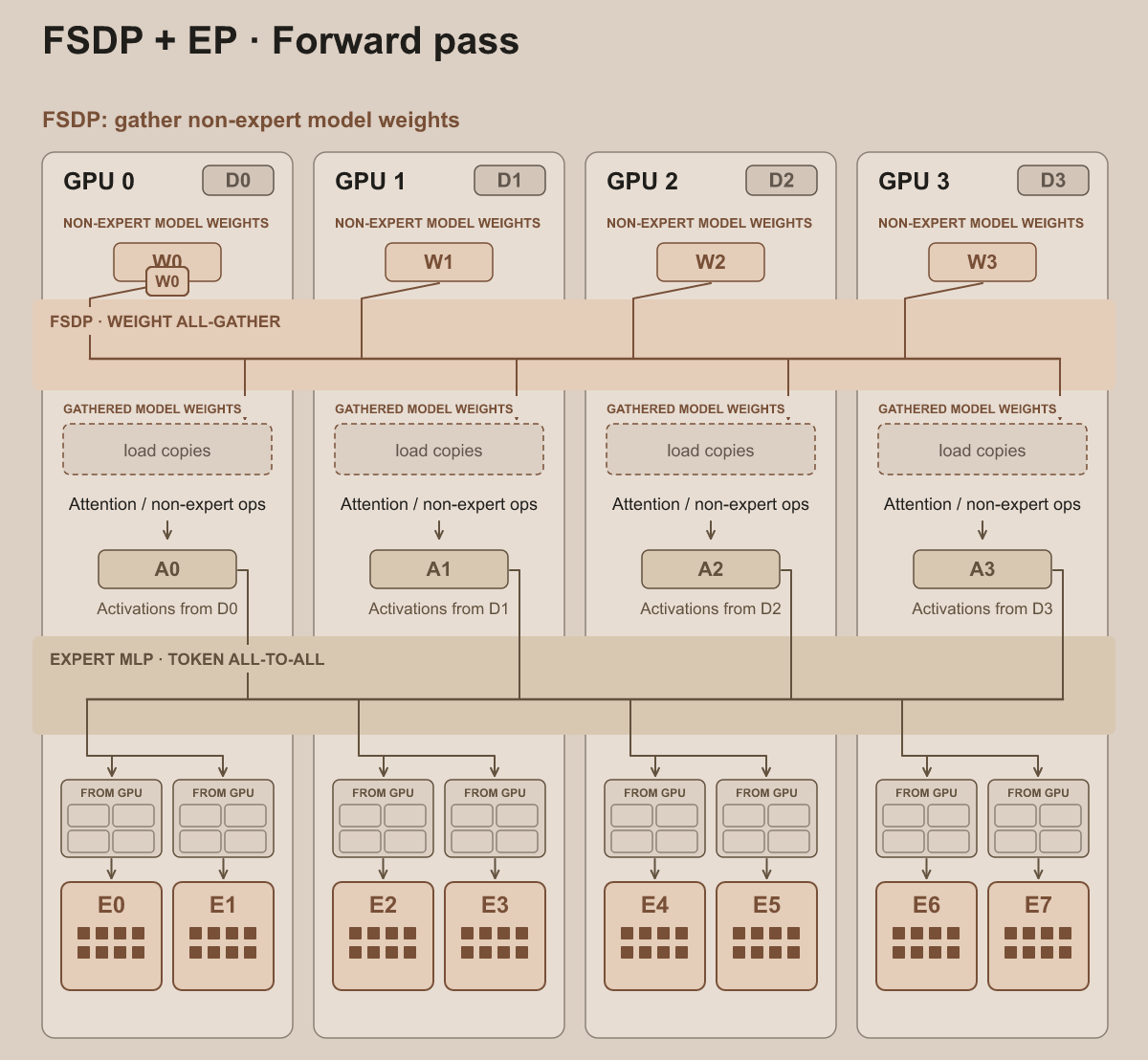
Going forward, when we say "tokens", we mean the token vector representation that flows through the LLM layers. In the context of EP, “dispatch” is the transfer of the tokens to their assigned expert; “combine” returns the expert outputs to their source GPUs and combines them into the layer output (see Figure 1).

Issue #8435 describes the full 535B-A23B model architecture. We use LatentMoE to reduce EP communication by projecting routed tokens from dimension 6,144 to dimension 3,072 before dispatch. This halves the token payload for routed expert dispatch and return. Of the 384 routed experts, eight are active per token. Two shared experts process every token. Routed expert weights are EP sharded, and shared experts and most of the non-expert weights are FSDP sharded.

Consider the 535B-A23B variant, a batch of 1,024 sequences per rack, sequence length 4,096, and 64 GPUs. It uses top-8 routing and 3,072-dimension BF16 token representations. Suppose we want to compare FSDP vs EP sharding for the routed expert weights, using back-of-the-envelope estimates with balanced routing. These estimates exclude padding, metadata, and backward communication.

For this same model shape, an FSDP forward pass would send approximately 20 GiB of routed expert weights per GPU per layer. EP requires approximately 6 GiB per GPU per layer for dispatch and combine. At fixed top-k, token width, token count, and GPU count, more experts increase the FSDP communication cost without increasing the EP token payload. See How To Scale Your Model: Transformer Accounting for more details.

From ragged-all-to-all to fixed capacity

In an MoE architecture, a learned router assigns tokens to experts. The number of tokens assigned to each expert varies with the router weights and the data. Which communication collective can handle these variable token assignments efficiently? How does the implementation handle routing imbalance?

Specialized EP communication libraries include DeepEP, Hybrid-EP, NCCL EP and MoonEP. There are also MoE megakernels such as Mixture-of-Kittens. Most were not directly usable in our JAX/XLA setup.

Ragged-all-to-all is a communication collective that supports variable-sized data slices, which suits EP communication. Our initial experiments reached only 15% MFU, despite recent performance improvements in OpenXLA. Further experiments exposed unexpectedly slow transfers, failures and NCCL hangs. These early experiments used a different model and precision configuration, so the later MFU results do not isolate the gain from the communication kernel.

After we collected profiles of the training steps, it was clear that we were not saturating the intra-rack network. The computation and communication overlap was far from optimal. We communicated the ragged-all-to-all performance issues to NVIDIA and proceeded to experiment with a custom EP communication kernel.

In a serendipitous turn of events, our GPU allocation arrived earlier than expected. Our updated plan was to support the best model shape at a non-embarrassing minimum of 20% MFU. We would kick off the hero run as soon as possible and improve the kernels during training. To that end, we created a custom EP communication protocol to support the 535B-A23B shape.

Our custom EP communication kernel, fixed-pooled-wave-all-to-all², reserves static capacity for the token assignments. Each sender GPU reserves one pool per destination GPU, and the six local experts³ share the pool. The pooling allows busier experts to use transport slots that quieter experts do not use.

The capacity factors control how much extra buffer to allow for imbalance. Each factor multiplies the assignment count expected with balanced routing. Sender capacity applies per sender–destination pair, and receiver capacity applies per expert, across all senders. Senders drop token assignments when the destination pool is full. Receivers drop token assignments when the expert capacity is full. A higher capacity factor reduces drops but increases memory use and communication overhead.

Receivers take incoming assignments in round-robin order across source GPUs to reduce bias from sender order.

Fixed sender pool and expert capacities allow us to use battle-tested and efficient all-to-all collectives and General Matrix Multiply (GEMM) for the MLP computation. We carry local expert IDs in the activation payload, so the receiver can group rows by expert without a separate metadata collective.

Finally, the dispatch and combine happen in 3 token waves to reduce the memory footprint. We size the sender and receiver buffers for one wave at a time. XLA may overlap parts of the waves as it schedules them. The unintentionally overly verbose name hopefully is somewhat self-explanatory by now.

We found agents effective for kernel development when they had a clear goal to hill-climb and feedback loops from tests and performance measurements. We integrated XProf and Nsight Systems profiling into the trainer and hosted the XProf viewer on Iris. We defined validation gates, from local tests through small-scale experiments to full-rack runs. We interrupted the inner agent development loop multiple times to steer the agent towards specific experiments, for example to avoid an extra metadata collective and to pack expert assignments along with the tokens.

On a single rack and with a 4k sequence length, we reached approximately 256k tokens/s, with median MFU of 24% and median assignment drop rate of 2.4%⁴. These medians cover the final 50 steps of a 200-step run, with sender capacity factor 1.05 and receiver capacity factor 1.33.

Does token dropping offset the capacity advantage?

The token assignment drop rate is the fraction of the token-expert assignments dropped due to capacity overflow. When an assignment for a given input token is dropped, the output token still receives contributions from the surviving expert assignments, the shared experts, and the residual path. In our experiments, longer sequences increased the drop rate at a fixed number of input tokens per GPU. Tokens in a single sequence tend to select the same experts.

We had an efficient EP+FSDP configuration for the 535B-A23B model, with a small but non-zero token assignment drop rate. The alternative was a dropless FSDP-only configuration for the smaller 360B-A23B model. Despite our reasonable expectation⁵ to improve both the efficiency and drop rate, we needed to understand the worst-case scenario of no improvements. Would the observed drop rate offset the capacity advantage of the larger model?

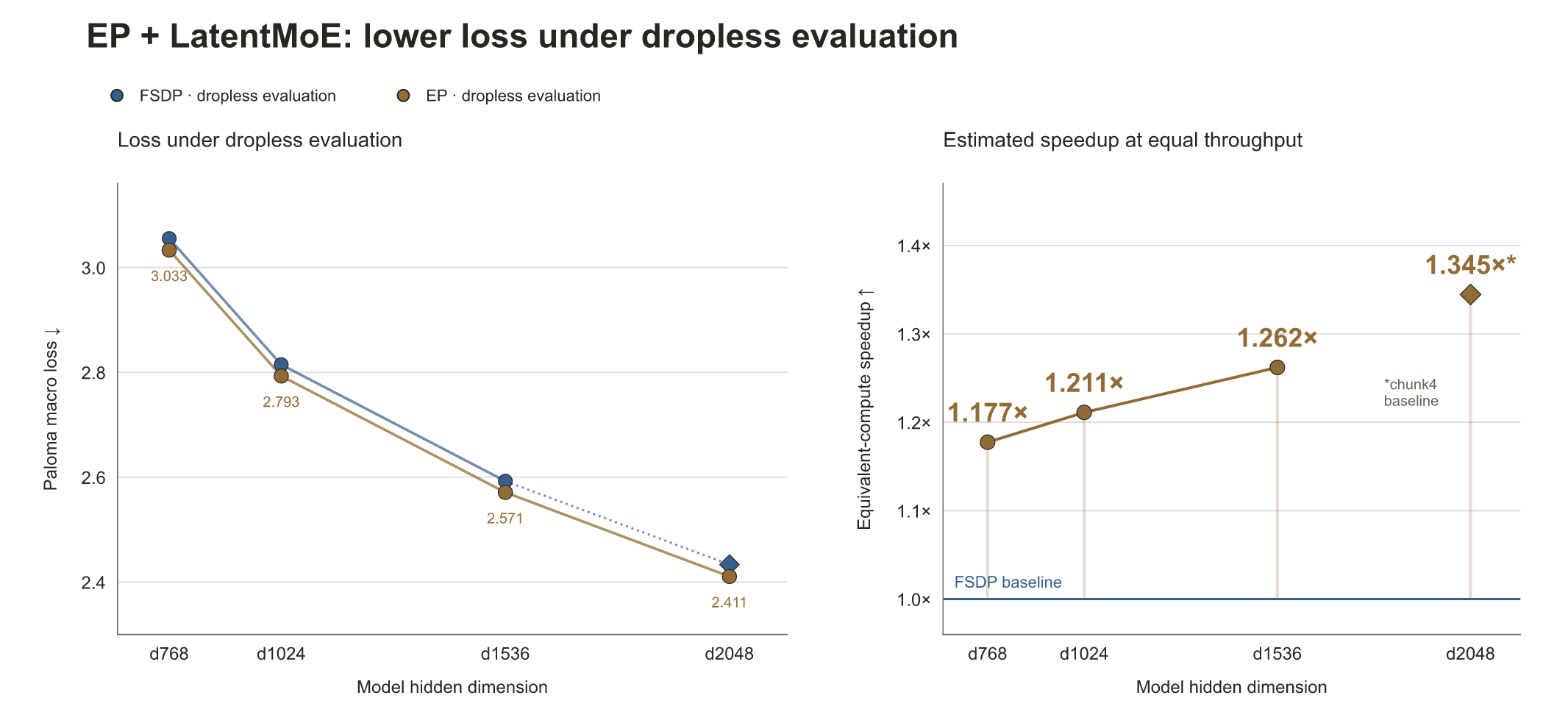
A four-rung scaling ladder experiment (54M to approximately 1B active parameters) compared smaller FSDP models with larger EP + LatentMoE models. We kept EP degree, batch size per rack, and sequence length at the anticipated hero-run values to approximate its token-dropping behavior. This ladder used an earlier model shape and fixed-all-to-all implementation, before the final 535B architecture and pooled-wave protocol.

Under dropless evaluation⁶, EP + LatentMoE achieved lower loss at every size, despite training assignment drop rates of approximately 5.5-7.1%. Under an equal-throughput assumption, the loss differences corresponded to an estimated 18–35% compute-efficiency gain over the FSDP baselines. Our loss-scaling formula estimates that FSDP would need 1.18-1.35x the compute to reach the EP loss.

View the full scaling ladder results.

These results supported our decision to select EP. They showed a loss advantage for the larger models despite assignment drops in the tested configurations.

From fixed capacity back to ragged-all-to-all

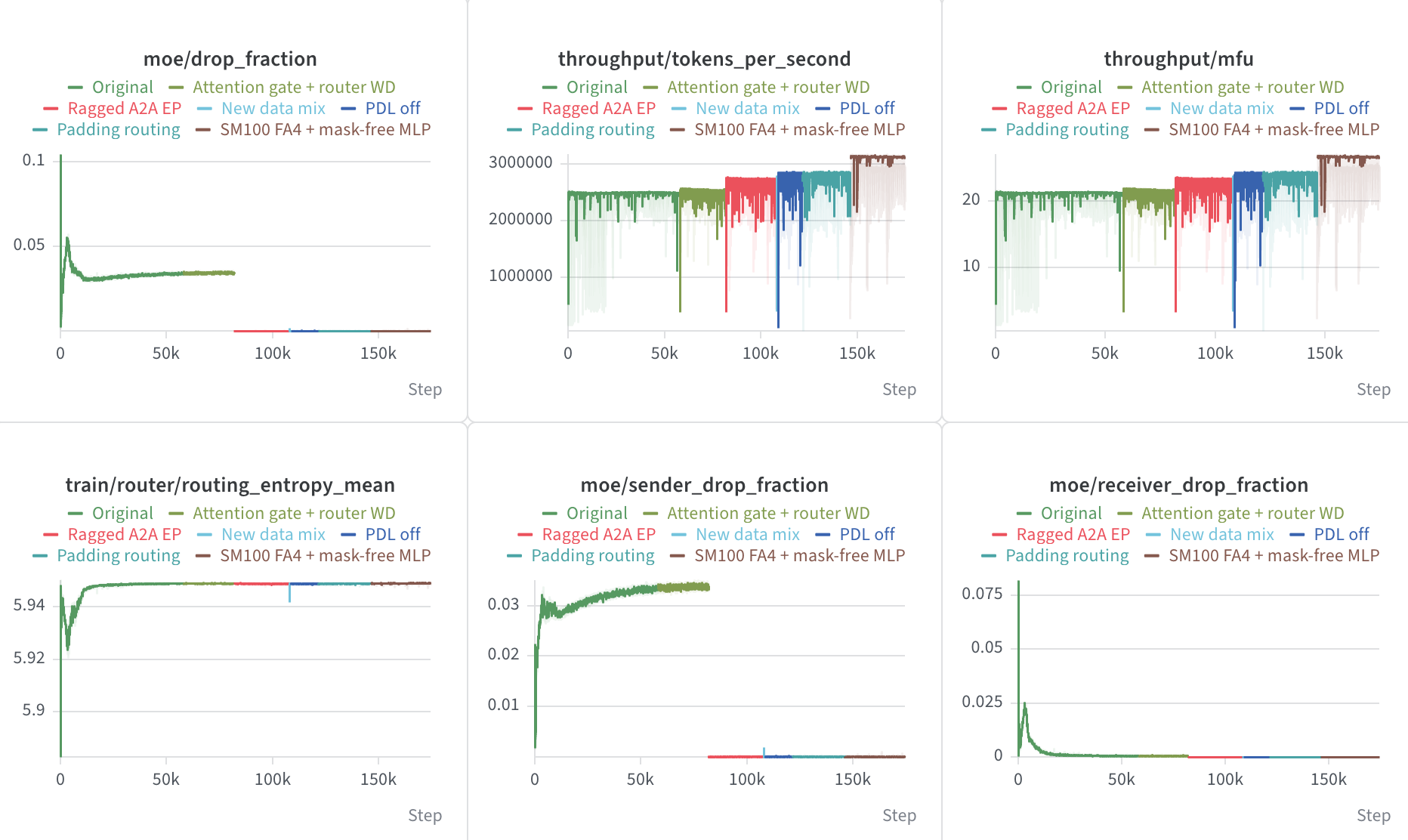
Fixed-capacity EP made the 535B-A23B model practical to train, and the scaling ladder supported accepting a small assignment drop rate in exchange for greater model capacity. The 535B-A23B-18T-Token-Hero-Run is a public WandB report of the hero run.

View the full metrics screenshot.

In the drop fraction pane, you can see the assignment drop rate settle around 3.5%. Most drops came from the sender pools. Receiver drops fell close to zero early in training, while routing entropy remained roughly stable afterward. The fixed-capacity kernel sustained approximately 21.5% MFU during production training.

In the meantime, Matt Wittmann worked on fixing ragged-all-to-all. Around step 82k, we switched to improved ragged-all-to-all. Assignment drops fell to almost zero, while the MFU increased to approximately 23%. Further changes were made along the way. We plan to describe the ragged-all-to-all fixes and subsequent improvements in a future post.

Contributions and acknowledgments

• Rafal Wojdyla: Implemented the initial EP experiments and profiler integrations, evaluated EP communication kernels, and implemented the custom EP kernel. Integrated EP into the hero model. Prepared this post and its figures.
• Matt Wittmann: Implemented the production ragged-all-to-all backend and subsequent performance improvements, which saved us weeks of compute time.
• Larry Dial: Designed and ran the EP vs. FSDP scaling ladder experiments, which enabled the final decision. Implemented the receiver-overflow rotation.
• Will Held: Helped design the FSDP and EP experiments.
• Mark Muchane: Ported the MoK megakernel and evaluated it in Marin.
• David Hall: Developed early EP implementations and correctness fixes, including ring EP, ragged-all-to-all, and DeepEP integrations.
• Russell Power: Ran ragged-all-to-all experiments and improved infrastructure performance.

We thank Larry Dial, David Hall, Will Held, Isaac Hodes, Percy Liang, David Lundgren, Mark Muchane, Ahmad Qamar, Matt Wittmann, and Romain Yon for feedback on this post.

@misc{wojdyla2026_expert_parallelism,
  author = {Wojdyla, Rafal},
  title = {Expert parallelism at hero scale},
  year = {2026},
  month = {sep},
  howpublished = {\url{https://www.openathena.ai/blog/expert-parallelism/}},
  note = {Open Athena Blog}
}