Scaling Samudra: Our journey towards better ocean emulators

What value lies at the center of science? I argue that it is not “truth,” nor is it “knowledge.” “Curiosity” comes close, but I feel that the value is resonant across many disciplines, like history or art. I contend that the core value that drives scientific inquiry is humility. The scientific method involves rigor and skepticism on the basis that it’s really hard to know anything at all. The goal to create knowledge where before there was none is inherently grandiose. Thus, to counteract such an ambition, one has to be vulnerable to the chance of being totally wrong. Therefore, science is about balancing doubt while being open to possibility.

To explain what I mean in the concrete, let me tell the story of how we arrived at our latest publication, Samudra 2, a neural ocean emulator. The core of our contribution in this work is how we were able to scale Samudra to emulate high resolution ocean simulations. If there is anything that I’ve learned about system optimization, it’s that it’s a humbling process.

I’ll briefly summarize our accomplishments: we extended the Samudra model to emulate an ocean dataset 16x the size of the original data (in bytes) with the same hardware budget. In this process, we reduced training time from four days to four hours on the original resolution. As we did this, we took the opportunity to introduce modeling changes that improved Samudra’s predictive skill, addressing several known problems in the first version of the model—a topic best understood through our paper website.

I’ll share how we achieved these milestones and the hard won lessons we learned along the way. But to better understand the context, let me explain our domain of research and the problems at hand.

Samudra in a nutshell

Why should you care about climate emulators?

Climate and weather models have a problem writ large: they’re very computationally expensive, and thus, we can’t simulate many impactful scenarios. For example, the ocean simulation we emulate requires over 4,600 CPU cores and can only achieve 12 simulated years per day (SYPD). This CPU allocation would consume about 15% of NYU’s entire super computing budget. This makes it very difficult to estimate outlier climate conditions, which may require thousands of simulated years to accurately calculate. Machine learning provides for us a way to rethink simulation and speed up estimates by orders of magnitude. Better climate prediction means we can help estimate (and then hopefully, mitigate) climate risks like extreme weather. Research in this area might one day help us identify climate tipping points or help guide interventions in the climate, like mCDR scenarios.

There’s a useful idea from computational science that captures why this is so limiting – time-to-solution: this is the total wall-clock time to move from scientific question to usable answer, not merely how fast a single model runs (or whether the model is neural or numerical). For the questions that matter most, like characterizing rare events or running large ensembles needed to pin down outlier conditions, time-to-solution is the real bottleneck. This is exactly where emulators shine: they collapse months of supercomputer time into hours on a single GPU, thereby making impractical experiments routine.

What is Samudra?

Samudra, named after the Sanskrit word for “ocean”, is a machine learning model that estimates the physical ocean across long time ranges. We predict the sea surface height, horizontal velocities, temperature, and salinity from the surface to the deep ocean. Samudra emulates the OM4 numerical simulation, which is the ocean component of the IPCC-commissioned CMIP6 project–a global, coupled climate model.

Samudra v1 training took 4 days on 8xA100s. It is able to simulate 100 years of ocean states at ~1152 simulated years per day, 100x faster than the base numerical simulation that powered OM4¹. Already, the Samudra class of models changes the equation: before, only governments or research institutions were able to make predictions about the ocean; now, small teams or individuals can. Our research begins with the question: can we do better?

Why should we scale across resolutions?

The Samudra v1 model is only able to emulate a 1°x1° representation of the base ocean simulation, whose full resolution is about a ¼°x ¼° grid², or 16x the number of grid points. By addressing the engineering challenge of making a more efficient training process, we are better able to make more skillful predictions. Furthermore, by investing in training efficiency up front, it makes us more suited to produce ocean emulators at higher resolutions and time spans than can be simulated with today’s numerical climate models.

How is Samudra trained? How does Samudra work?

Samudra is a physically-informed CNN. That is, we use a base understanding of physics to structure a machine learning problem such that a neural network is likely to succeed. Specifically, Samudra is a convolutional U-Net. Its base blocks are inspired by ConvNeXt UNets, though Samudra makes use of standard dense blocks with dilations rather than depthwise convolutions³.

Samudra is an autoregressive model: we take the state of the ocean at time t₀ and predict time t₁. Then, we feed that output, t₁, back into the same model to predict the next time step, t₂. We do this over and over again in a “rollout” over a long time horizon. In our work we are able to achieve a stable Samudra model for an 8 year rollout, where each time step (dt) is five days.

The previous state of the ocean alone is not enough to know what will happen next. This is because the ocean system is dependent on what happens in the atmosphere (let alone the land and sea ice) – they are a coupled climate system. We call the influence of the atmosphere on the ocean a “forcing”. Our model is designed to take in atmospheric forcing information (representing the ocean-atmosphere boundary) as an oracle during the training process. This design element makes it easier to couple neural emulators with general circulation models (GCMs) or other emulators – see SamudrACE.

Any dynamical system like ours faces a common problem: when predictors feed back into themselves, even the tiniest amount of error tends to accumulate fast. Very quickly in the rollout process, we’re liable to produce grossly incorrect forecasts, even if the model does well at predicting one timestep to the next. Our training process is designed to mitigate this tendency: Instead of taking the loss against one step of predictions at a time, at each training step, we perform a mini rollout of N steps. Aggregating the loss over several steps⁴ tends to make the model aware of the consequences of errors in the earlier prediction steps in the rollout.

Scaling Samudra

Now, I’ll explain how we tuned the system performance of the Samudra model – in four acts.

Act 1: Data Loading

Our first goal was to see if we could significantly reduce training time. If we could get each training run down to less than one day, then it would give us a larger experimentation budget to address the outstanding modeling problems.

The first place we thought to look was in the data loader. (The problem is always the data loader, isn’t it?) To start, we did some profiling with the PyTorch Profile (on 1xA100). This is what it revealed:

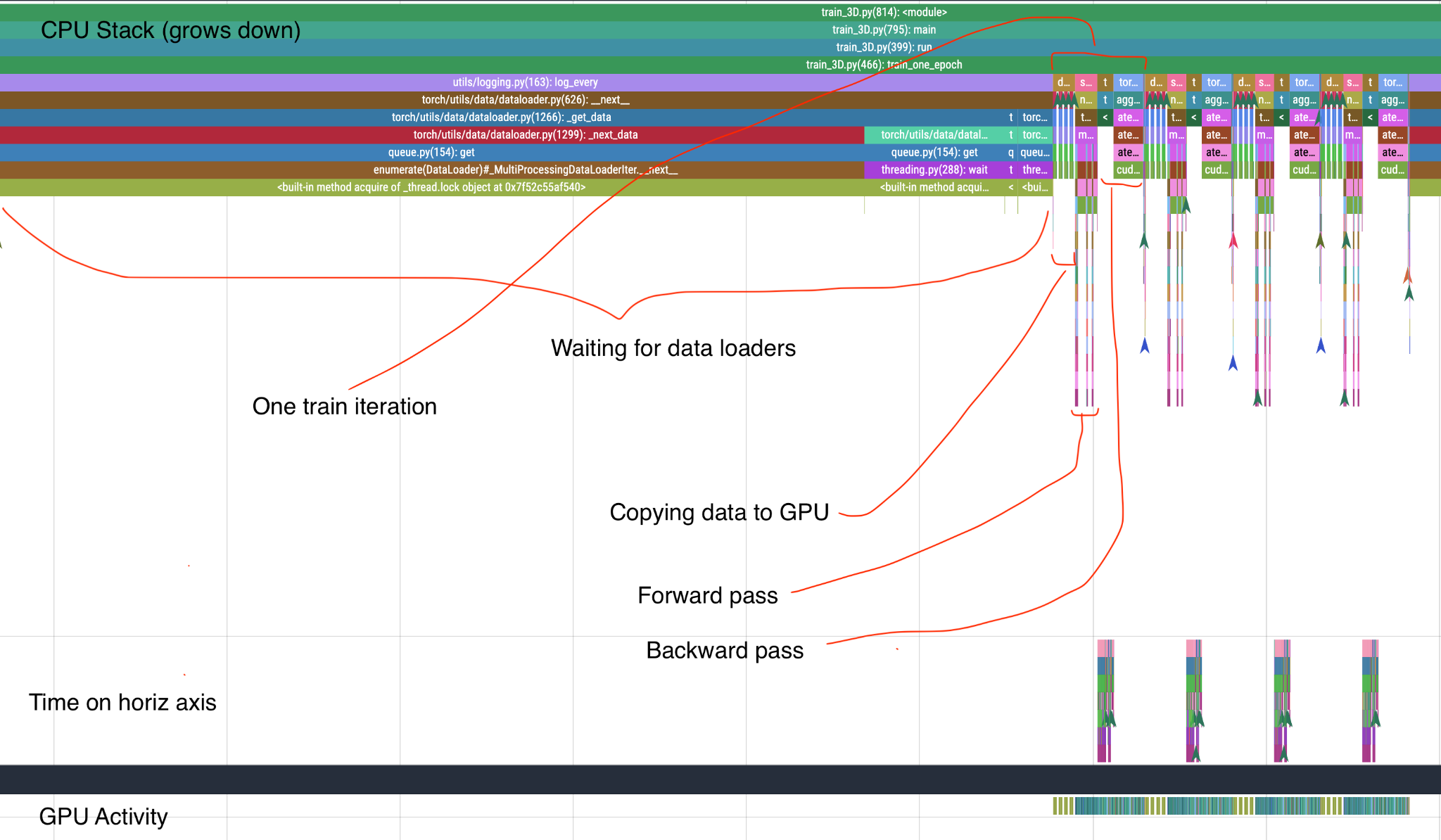
Our initial assumption proved correct: for one training iteration, orders of magnitude more time was spent waiting for the data loader before the GPU was ever made active. All GPU related activity – copying data to GPU, the forward and backwards passes – were miniscule by comparison. Upon further profiling of the data loading processes, it seemed like Dask, the default Xarray backend, might have been contributing to this slowdown. We had heard from peers that one should always turn off Dask inside the training loop: there’s no need to build the task graph (for streaming analytics) when all we need to do is move bytes from disk to device. From here on out, we disabled Dask when we opened our Zarr dataset in Xarray.

While PyTorch produced very complete traces of what was going on in the system, it was a bit unwieldy to use: Profiling produces huge traces (30 seconds of model execution including stack traces produced 2GBs of JSON) – so much so that the standard visualization tool – Perfetto – struggled to load them.

Given this, and the fact that most of the time spent did not involve GPU at all, we switched to profiling with PySpy, a relatively new statistical profiler in Python (backed by Rust). Unlike Python's native cProfile tools, PySpy gives us both native and Python-level stack traces and can include subprocesses. We reran training with py-spy record –native attached and got a very interpretable SVG that diagnosed the problems in the data loader:

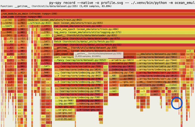
Reading these traces, we found that the actual code performing any data movement was the very modest box inside the blue circle (above). The rest of the operations inside the _getitem__ call (the tooltip shows this represents ~83% of all samples) was pure Xarray overhead⁵. That I/O is actually only a tiny part of load times was a surprise.

Takeaway: commonly used libraries may not be appropriate for your use case, especially within tight loops. In our case, we needed to be more skeptical of Xarray and Dask.

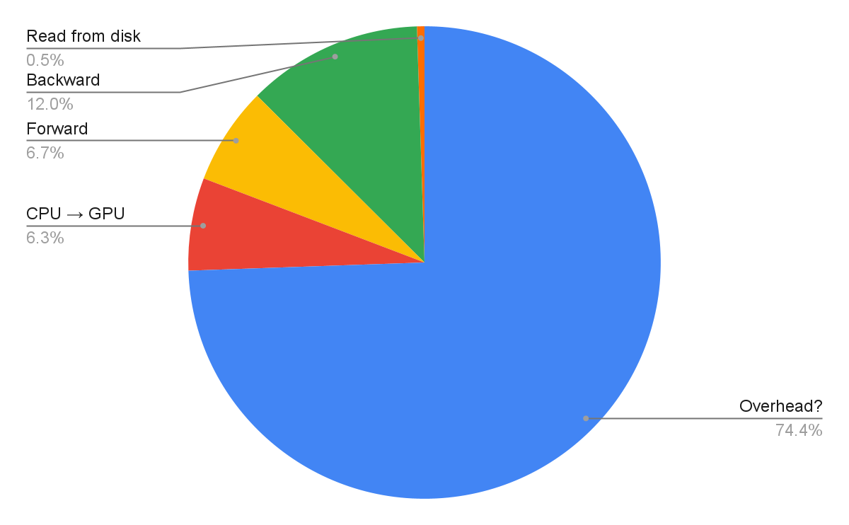
Given the output of these two profiling tools, we found out that 75% of each training step was spent waiting for the data loader. Thus, we set our sights on speeding up the data loader, and we felt confident that this would solve our large training time problem. To this end, we conducted many systems experiments.

Approach 1: Disabling Dask

As I mentioned before, we disabled Dask to eliminate the task graph build times. Unfortunately, this exercised less-used paths within Xarray, so we ran into bugs that made it easy to accidentally use much more memory than expected. After some small work-arounds and an upstream patch, our Dask-less data loader was stable and significantly faster than our original pipeline.

Approach 2: Chunk optimization

The canonical way to address systems performance problems in the Climate & Weather community revolves around a single concept: chunks⁶. Once we simplified our set of system components, this is the next knob we attempted to tune. It seemed reasonable to us that if we increased the chunk size across training examples (to load more examples into memory from disk at once – specifically, increasing the time chunks from 1 to ~10), we could batch I/O overhead costs to speed up our pipeline. To our dismay, this made things slower. Our reasoning behind this, and why we must set chunks=dict(time=1), is that we use random access across time due to the random shuffle used during ML training. When loading larger chunks, we ended up pulling contiguous time slices of data from disk into memory that we immediately threw away. A possible solution we considered to take advantage of optimal chunk slicings was pre-shuffling our training data, but we opted against this for various reasons⁷.

Approach 3: Data structure tuning

Our next experiment involved a bit of data engineering: Our 3D ocean variables are stored separately for each of 4 physical variables crossed with 19 depth levels, making 76 total variables. We sought to re-shape our Zarr store to be "canonical", meaning just 4 variables with a depth dimension. The theory for why this should help, we thought, was that it was a simple way to reduce I/O overhead: it should be a win to make 19x fewer loads from disk and then process them to a ML example within memory. To our surprise, this did not help at all either. One reason for this could be that modern SSDs and OS kernels are surprisingly efficient at I/O compared to the overhead of additional data manipulation. Maybe if we were loading from bucket storage, this would be a win – alas, it was not.

Approach 4: Concurrency

At the time we were conducting these experiments, our profiling revealed a serious performance bug within Xarray (that since has been patched): while in theory all data_vars in an Xarray Dataset could be loaded in parallel, the way it was implemented, it loaded serially (!!). Since our OM4 dataset includes 19 x 4 + 4 (=80) data variables, this is an unnecessarily long time to wait! We intervened by setting up a thread pool via concurrent.futures where we ran DataArray.compute on background threads. Luckily, this did speed up loading data from disk!

Approach 5: Vectorized loading

The next optimization we suspected was worthwhile involved vectorization with Xarray. As I mentioned in the background, each training example doesn’t contain a single timestep of data, but rather, four (input and output pairs). In the status quo, we had a big for loop to select the slice of data that we needed. This seemed inefficient in comparison to, say, calculating the indexes for all the data we would need across all steps and then making one query of all the data output as a single array. However, when we implemented this and compared the results to the status quo, it actually made things slower compared to a standard Python loop + successive Dataset select statements! While we were examining this area of the data loading loop, we did try something similar: we re-wrote the select statements in Xarray to reduce the indexing burden per lookup. This did help, on the other hand.

Synthesizing the improvements

All of these incremental changes added up, and our new data loader benchmarked to be 5x faster than before (in our benchmark test setup). Here are the differences to our data loader (in pseudocode) at the start and end of our optimization process:

#
# Before optimization
#
data = normalize(xarray.open_dataset(path))

def __getitem__(self, idx: int):
  result = TrainData()
  for step in range(self.steps):
    time_index = self._get_time_index(idx, step)
    prognostic_in = (data[prog_vars]
                     .isel(time=time_index)
                     .isel(time=slice(None, 2)))
    prognostic_out = (data[prog_vars]
                     .isel(time=time_index)
                     .isel(time=slice(2, None)))
    result.insert(
      prognostic_in.to_array().to_numpy(),
      prognostic_out.to_array().to_numpy())
  return result

#
# After optimization
#

# Disable dask
data = normalize(xarray.open_dataset(path, chunks=None))

def __getitem__(self, idx: int):
  result = TrainData()
  for step in range(self.steps):
    time_index = self._get_time_index(idx, step)
    # Get all prognostic data at once
    prognostic_all = data[prog_vars].isel(time=time_index)
    # Force compute on background threads
    concurrent_compute(prognostic_all)
    # convert to torch, _then_ normalize 
    result.insert(normalize(torch.from_numpy(prognostic_all.to_array().to_numpy())))
  return result

Before improvements (first snippet above) – things to pay attention to:

• We normalized the data immediately after loading using Xarray and Dask. This incurs building a Dask graph. Since Dask is lazily evaluated, it meant we were probably calling normalization code before each load anyway, but with the overhead of the Dask graph.
• We loaded the input data t0 and target t1 separately.
• We passed around NumPy arrays and converted to torch late (as is standard, in the collate function).

After improvements (second snippet above) – aspects to notice:

• Dask is disabled, and we found it was better to normalize late instead of up front.
• We can reduce indexing overhead by selecting all the ocean data (“prognostic”) up front and dividing it into t0 and t1 inputs/outputs late/in-memory.
• We didn’t depend on a future Xarray improvement and instead forced it to load each xr.Variable before we proceeded, and wrote a one-off method to compute each variable concurrently.
• As soon as possible, we loaded the data to PyTorch, and then normalized it there.

Now, with a better data loader in hand, it was time to see what all this hard work amounted to – we re-ran a training run to see how much time it saved. The results amounted to the following:

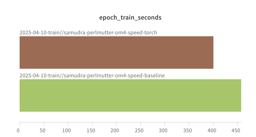
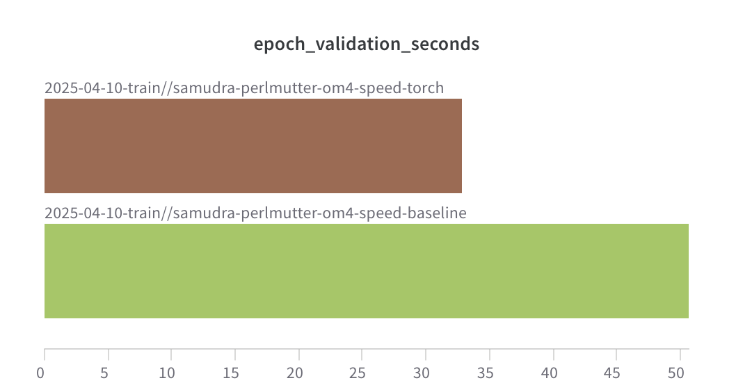
Ok, the time is better but … not much better? This, indeed, was a surprise.

Takeaway: Profile on the actual training set up, not just the micro-benchmarks.

What was going on?

Act 2: Inference

Meanwhile, on real hardware, inference (i.e., the autoregressive rollout) was run during training. This was included so that per each epoch, we could examine the performance of the model with a realistic scenario. It makes scientific sense to prove the model works at longer time horizons instead of the meager four steps we backpropagated against during training. However, this apparently came with a steep cost: inference took up a large fraction of train time.

Our colleague (Surya Dheeshjith, the lead author of Samudra v1) made an update to log experiment results less frequently during inference. This, to our surprise, made the overall pipeline 4x faster! This routine change led to 4,800 SYPD for inference (at 1°), and had a much larger impact on training time.

Takeaway: When profiling a system, zoom out before optimizing.

Even with this 4x improvement, these inference steps interwoven with training still took a huge fraction of time. Inference occurs on a single GPU, which means that our 8xA100s were laying idle during the inference phases. These inference runs were diagnostic, and the most valuable verifications we could just run on saved checkpoints after training instead of during. Thus, our simplest optimization yet was to simply split the scripts to perform the rollout independently from the training phase.

Takeaway: do less when possible!

Act 3: Memory Usage

Now that we made some progress speeding up training, we could work on the next major system performance goal involved with scaling Samudra. Specifically, how can we make a model designed for 1° resolution train on data at a ¼°?

Before I discuss the difference implied by a higher resolution, let’s take a closer look at what 1° data looks like for training:

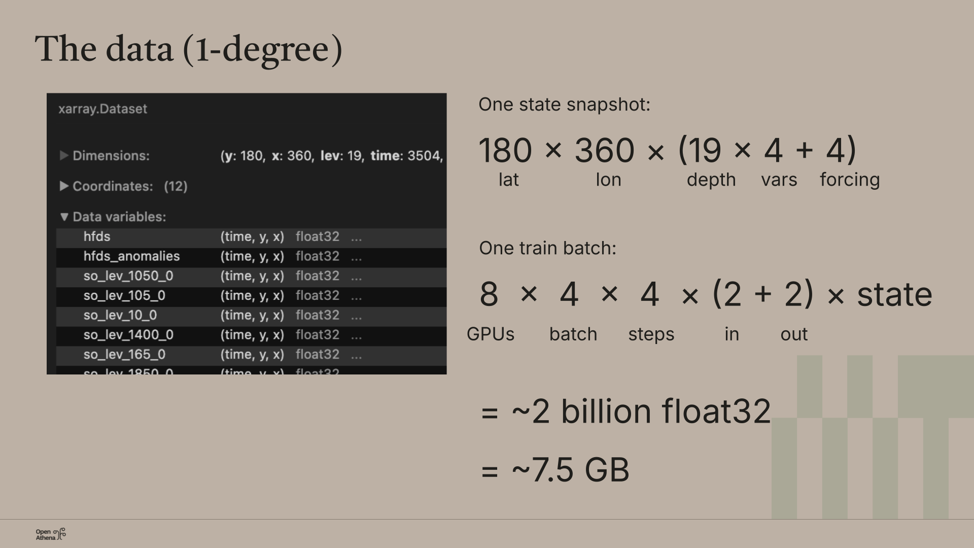
• Data is stored in Zarr, a cloud optimized data format, in uncompressed chunks. We load the data from disk onto the CPU. We load the data (and build mental models of it) with Xarray.
• One state snapshot of the data is composed of following: 180° latitude x 360° longitude x (19 depth levels * 4 variables) + 4 forcing variables (at the surface).
• However, training takes a composition of states in a batch. Batches are distributed on multiple devices of hardware, namely 8xA100 GPUs. Given this state, a training batch is defined as: 8 GPUs x 4 batch x 4 steps x (2 in + 2 out) x state. This amounts to ~2 billion float32 numbers, which amounts to ~7.5 GiBs per train step.

Given this as the basis of our training data, what would it cost to scale to ¼° data, using the same analysis?

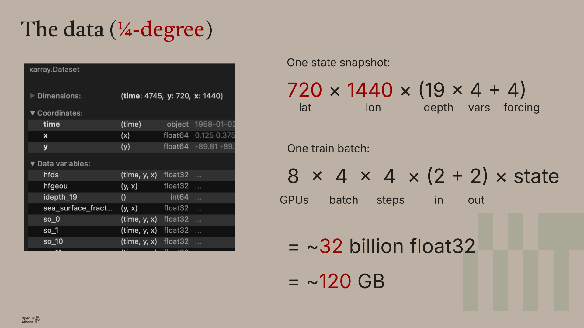
• State becomes 720 lat x 1440 lon x (19 depth levels x 4 variables + 4 forcings)
• This means that the same train batch with a batch size of 4 becomes ~32 billion float32 numbers or ~120 GiBs.

Per GPU, just the data would take up 15 GiBs of memory. However, when the data size increases, so do the stored activations within the forward and backward pass. Our A100s have only 80 GiBs of high bandwidth memory for us to work with. Without intervention, our model wouldn’t be able to handle this increase in memory.

To address this memory bottleneck, we began measuring how much memory the model was currently using. Our initial metric analysis looked like the following:

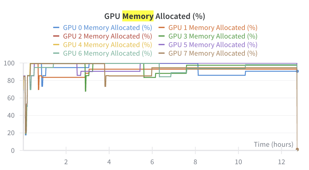
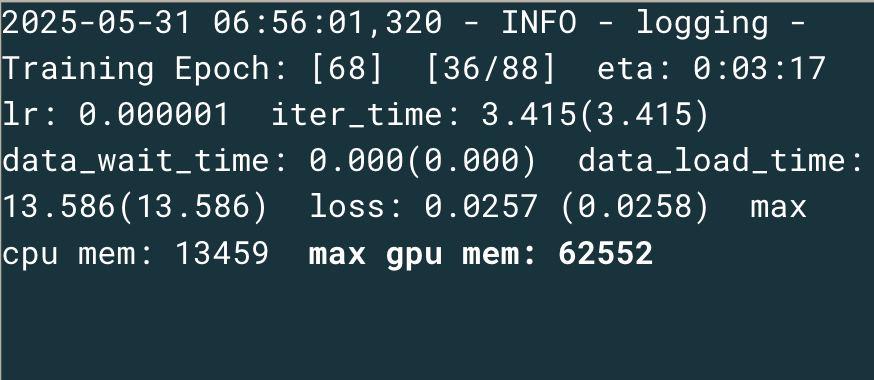
Weights & Biases, our experiment tracking system, reported that training allocated 100% GPU memory. We compared this number to logs we make every train step. These reported that memory grew to 62 / 80 GBs for the 1° run. We found this to be strange. Does the model really grow to 62 GBs and then never change? We re-ran a training run to see if this figure was consistent. It wasn’t. This next run reported 75 GBs of memory usage. Another run revealed 68 GB. What was going on?

The logs and W&B plots generally were coarse measures. We needed to see what was really going on here. To this end, we leveraged PyTorch’s CUDA memory snapshot profiling tool. Here’s what we learned from this tool:

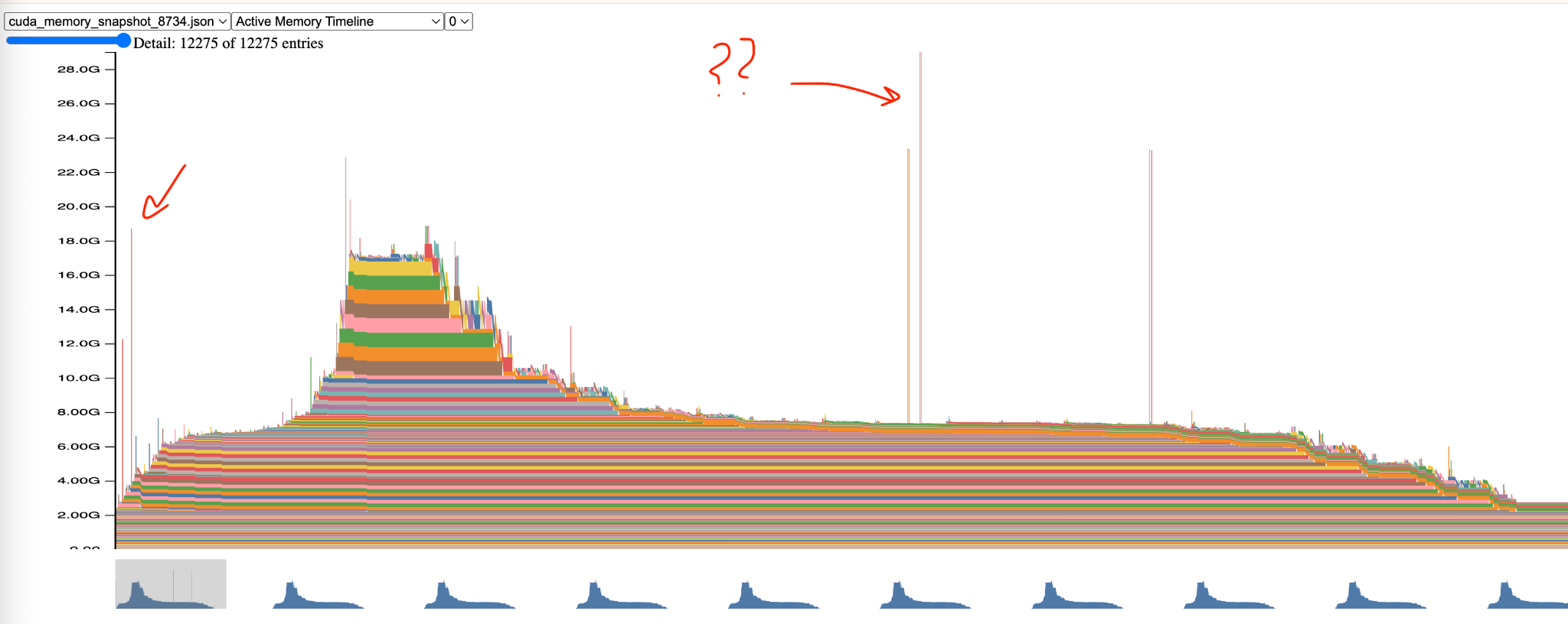
The first thing that jumped out at us: what were these weird spikes?? We dug into the backtraces of the allocation spikes above and discovered that PyTorch uses speculative allocations to discover how much memory is available before allocating memory for internal scratch buffers.

The “magic” behind the framework messed with our simple logging approach. Looking back at either trace, we found that W&B provided too coarse of a measure. The logs, on the other hand, performed a local max and never reset after the high watermark – a bug on our part. Thus, both these system measures were technically correct, but not useful to answer the question at hand.

Takeaway: Trust, but verify.

Now that we had detailed measures of the 1° training passes memory capacity, we could better ask: how could we address the memory limitation on our hardware to scale to a ¼° of our model? Many machine learners probably already know the answer: In our case, activation checkpointing saved the day.

What is activation checkpointing? Briefly, it’s a setting in PyTorch that lets you trade memory for compute. This means that the forward and backward passes will take more time, but it allows you to fit these activations within a fixed memory budget. Instead of storing activations in memory, as is standard, activation checkpointing will recompute them on the fly.

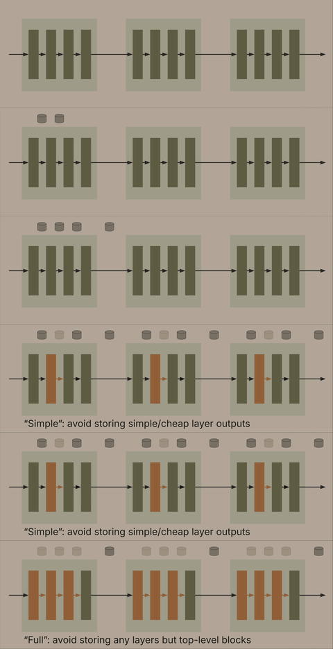
Here, we modified our model and created two experimental configurations. First, we created a “simple” mode of checkpointing activations: we would avoid storing everything except simple or cheap layer outputs, only re-computing the 2d Convs within each core block of our UNet. Second, we created a “full” checkpointing mode, where we recompute activations for everything but the top-level blocks. We then ran each path through a live training run, which we can characterize as follows:

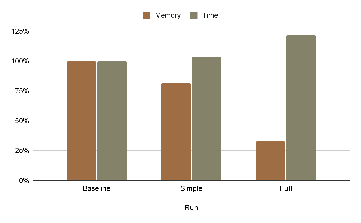
Compared to baseline, simple checkpointing gains us 20% more free memory for a marginal cost of time. However, full checkpointing buys us over 60% more free memory capacity for around 25% more time. We decided that full activation checkpointing was well worth the tradeoff. From here, we began experimenting with training on ½° data, which incurs 4x more bytes, using full checkpointing. Our efforts at ½° resolution, as luck would have it, would carry over to the full ¼° dataset.

Act 4: Return of the data loader

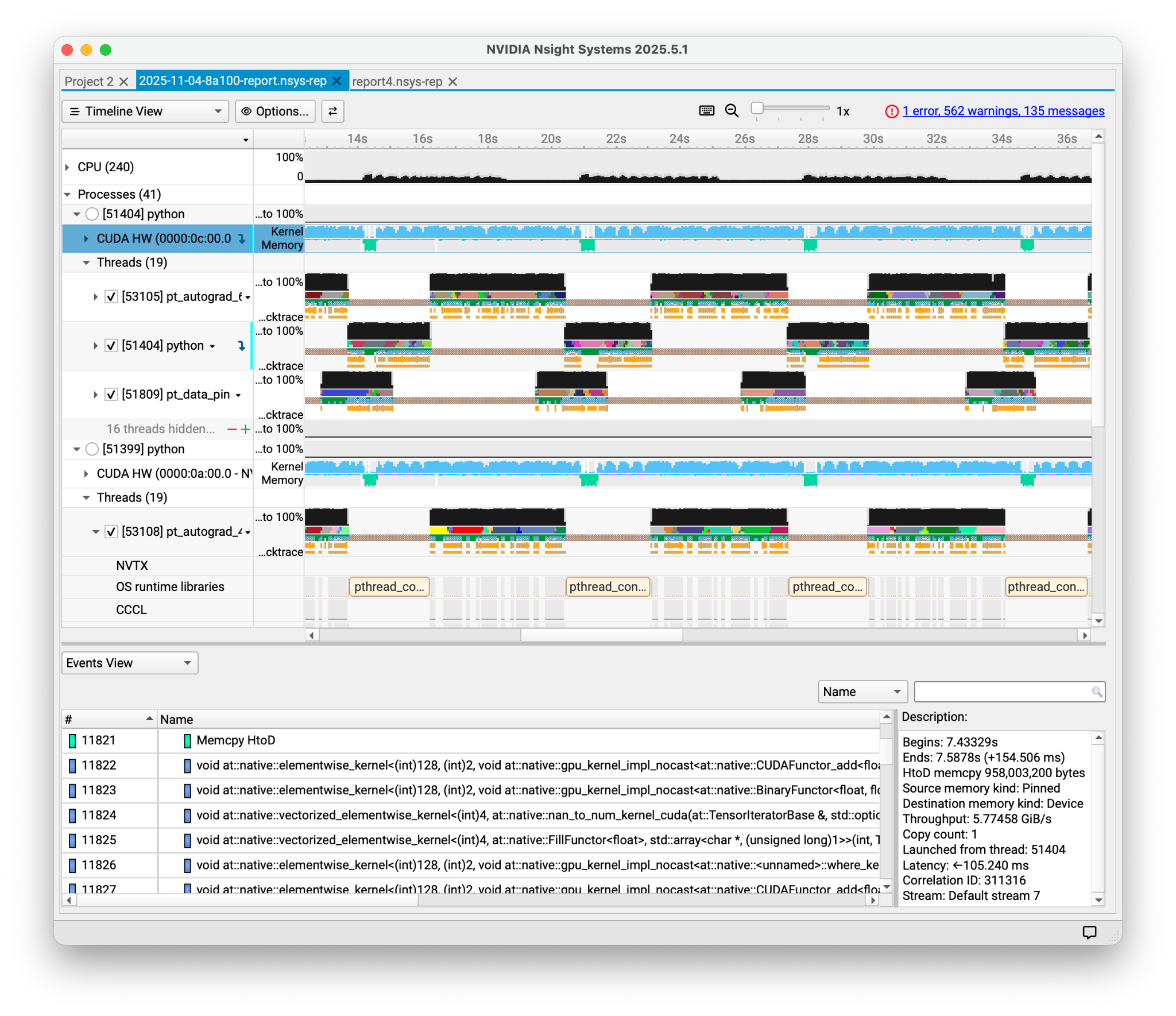
Taken together with the improvements to the data loader and by removing inference from the training pipeline, the GPU once again became the bottleneck for training on ½ degree data. This time around, to diagnose problems in our GPU utilization, we made use of NVIDIA’s Nsight Systems profiler. This tool is powerful, but can be difficult to get acquainted with. Luckily, there is a good course to get started. Further, NVIDIA’s friendly outreach folks helped us a lot, too (many thanks to the Higher Education and Research team).

Initial profiles with the tool revealed surprising data transfer behavior. Namely, a lot of memory we were trying to move to the GPU was not “pinned”, causing the transfer to be slow and block the CPU from doing other work.

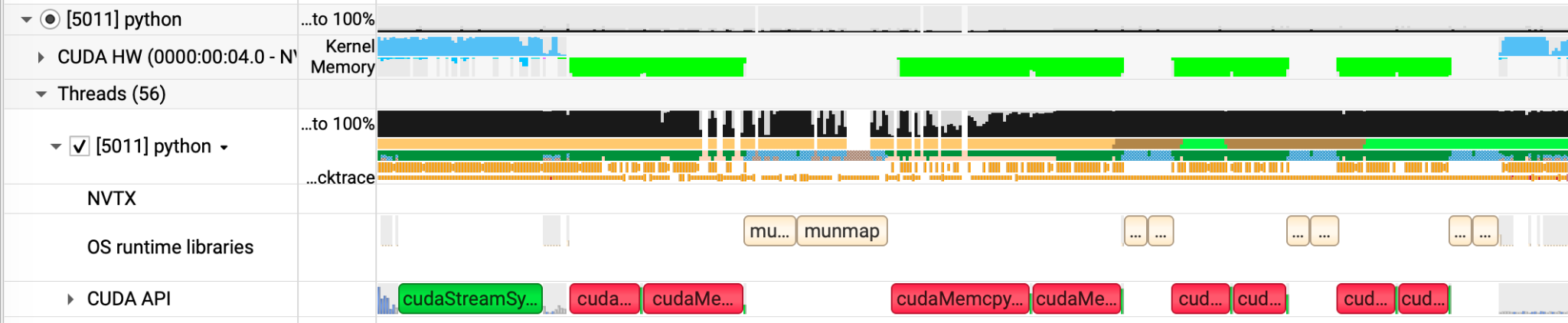
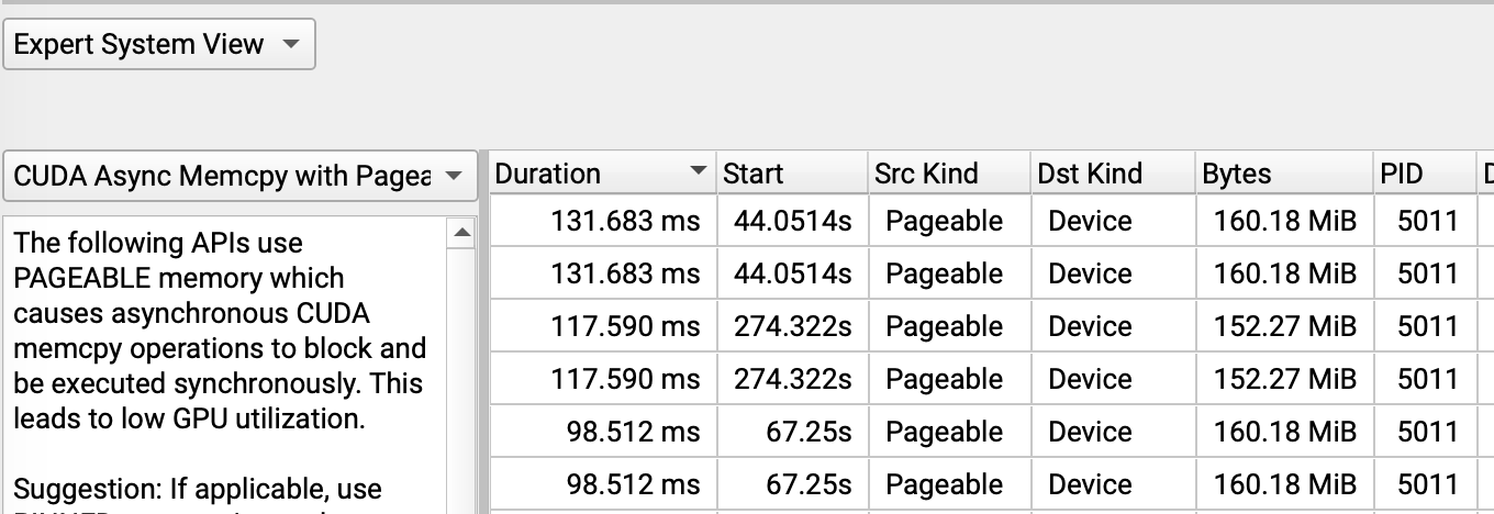
The fix was fairly straightforward, though we wouldn’t know to do it without using this profiling tool and reading the PyTorch docs: PyTorch will pin memory for arbitrary Python objects, but only if those objects have two methods available: to(device) and pin_memory(). By adding this to our core “batch” class, i.e. TrainData, and adapting it for our batch’s data model (we store tensors for every step of our rollout prediction), we were able to copy data from CPU to GPU way faster.

class TrainData:
  def to(self, device: torch.device) -> None:
    for step in self.steps:
      self.steps[step] = (
        self.step[step].to(device, non_blocking=True)
      )
  
  def pin_memory(self):
    for step in self.steps:
      self.steps[step] = (
        self.step[step].pin_memory()
      )
    return self

Running profiling with Nsight showed a win: in our test setup, we got a ~10-20% train time improvement. However, on real hardware, train time improved 2x!

Takeaway: removing bottlenecks can have surprisingly beneficial results!

Running the job for a while longer, it seemed that this improvement only lasted for the first couple of training steps? From profiling it again, we found out now the bottleneck was actually on the CPU side of data loading. We realized, the CPU side slowness was no longer the data transfer, it was performing normalization on the data right before load. That was slow on the CPU, and mitigated the effect of the improved data transfer.

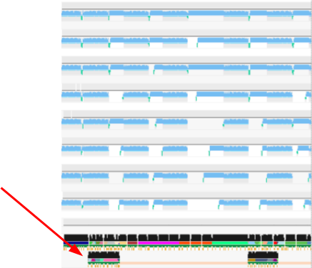
Takeaway: make sure to profile the actual training step (again).

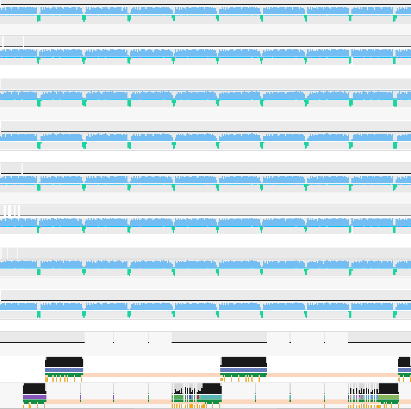
The solution to this was fairly apparent: We wrote code to move the normalization on to the GPU. This removed the gaps between memory copies where the GPUs were idle. Now, to the best of our understanding of the profiler, our GPUs were working as they should—which is to say, they were going brrrrr.

Samudra 2 in retrospect

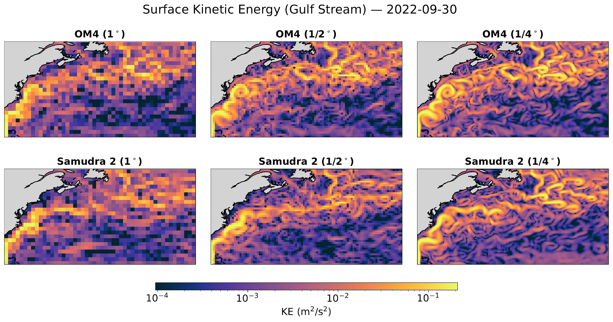
Overall, in this model release given our investigations within the permitted time, we accomplished the following:

• Reduced training time from four days to four hours.
• Inference grew 4x faster (totalling ~4800 SYPD).
• Gained the ability to train on 16x larger data in bytes.

With this new, hard won compute capacity, we were able to produce a more skillful model at resolutions that matter to make neural ocean forecasting practical⁸. Overall, we created a foundation that served our scientific investigation so far, and all research we will conduct in the future. However, the path here was not as easy as we would have expected.

A long held belief I have is that “there are no reliable narrators.” The engineering conducted here underscores this: nearly every time we made a confident hypothesis, we were proven wrong through measurement. Even when we knew to measure instead of guess, our tools sometimes told a version of the story that was unreliable. When every decision invites skepticism, it's a wonder that we can know anything at all. That realization, in my view, is why humility underpins all of science. While I don’t like being wrong, I have immense gratitude for all the humbling work that precedes me, and all that lies ahead. I am grateful for all those willing to be wrong perchance to learn, to know.

@misc{merose2026_scaling_samudra,
  author = {Merose, Alexander},
  title = {Scaling Samudra: Our journey towards better ocean emulators},
  year = {2026},
  month = {jul},
  howpublished = {\url{https://www.openathena.ai/blog/scaling-samudra/}},
  note = {Open Athena Blog}
}